
Before you read the answers
- A count that looks right is easy to produce and hard to verify. This guide gives you an order to practise in and a checking habit for every criterion you write.
All examples use original synthetic data. Source row numbers and column letters are shown so you can reproduce the formulas.
Checking a regional count against a filter
Count the rows for one region, then confirm the count by filtering the same column.
USD per unit and USD revenue. One fictional order per row, November 2026.
| Row | A · Order ID | B · Region | C · Channel | D · Units | E · Unit price (USD) | F · Revenue: your formula |
|---|---|---|---|---|---|---|
| 8 | RS-101 | East | Direct | 18 | 42 | Blank task cell |
| 9 | RS-102 | West | Partner | 12 | 55 | Blank task cell |
| 10 | RS-103 | North | Direct | 25 | 32 | Blank task cell |
| 11 | RS-104 | East | Partner | 16 | 48 | Blank task cell |
| 12 | RS-105 | South | Direct | 30 | 29 | Blank task cell |
| 13 | RS-106 | West | Direct | 14 | 55 | Blank task cell |
| 14 | RS-107 | North | Partner | 20 | 35 | Blank task cell |
| 15 | RS-108 | East | Direct | 22 | 42 | Blank task cell |
| 16 | RS-109 | South | Partner | 15 | 31 | Blank task cell |
| 17 | RS-110 | West | Partner | 10 | 58 | Blank task cell |
| 18 | RS-111 | North | Direct | 28 | 32 | Blank task cell |
| 19 | RS-112 | South | Direct | 24 | 29 | Blank task cell |
Worked solution and complete results
the row revenue for the first regional record · F8
=D8*E8Result: 756
the row revenue for the fifth regional record · F12
=D12*E12Result: 870
A mistake to catch
Writing the region name straight into the criterion without quotes, so the formula is rejected or read as something other than text.
Correction. Put text criteria in quotes, or hold the region name in a labelled cell and point the criterion at it with absolute references.
Read the result
If the formula count and the filtered row count disagree, the criterion or the range is wrong. Fix that before adding a second criterion.
What order should you practise COUNTIF and COUNTIFS in?
Before you write any formula, decide how you will check it. The habit that matters most is comparing the formula result with a filter using the same condition, and doing that on every new criterion until it becomes automatic.
Each step should use a fresh sheet or different data, so the answer cannot be memorised. If you are still building confidence with the single function, work through [the COUNTIF lesson](/lessons/countif/) first, then return here.
Use graded exercises to get cell level feedback, then rebuild the same formula from a blank cell later in the week. The gap is what turns a copied answer into a skill you can repeat under pressure.
Keep a one page log of the criteria you have tried and what each one returned. When a later count surprises you, the log shows whether the data changed or your criterion did, and that saves an hour of guessing.
- Count one text criterion and check it against a filter using the same condition.
- Repeat on different data so the answer cannot be remembered.
- Rebuild the formula from a blank cell a few days later.
- Only then open [the COUNTIFS lesson](/lessons/countifs/).
How do you write a criterion that Excel reads the way you mean?
Text criteria go in quotes, plain numbers do not, and comparison criteria are written as text with the operator first, for example greater than or less than followed by the value. Microsoft's COUNTIFS page documents the criteria syntax and comparison rules, so read it once before you start guessing.
When the criterion sits in a cell, join the operator to the cell reference rather than typing the value into the formula. Lock the criteria cell with absolute references when you fill the formula across or down, as covered in [the references lesson](/lessons/references/).
A criteria cell reference on its own compares against the value in that cell; when you need an operator, join it to the reference, for example with an ampersand, or the formula will not do what you expect.
Watch the quote marks themselves. A criterion pasted from a document can carry curly quotes that look identical on screen but are not read as text delimiters. Retype the quotes by hand if a formula is rejected for no obvious reason.
- Type the criterion you expect in its own labelled cell.
- Write the formula using the operator joined to that cell reference.
- Make the criteria cell absolute before copying.
- Change the cell value and confirm the count moves.
Which COUNTIF mistakes quietly return the wrong count?
Numbers stored as text, trailing spaces and non printing characters can make visible matches fail. The cleanup steps in [the imported data guide](/guides/clean-imported-data/) may help you deal with those at source; check that the guide covers the specific issue you have before relying on it, and do not repeat the fixes inside every formula.
COUNTIFS ranges must be the same size and shape. Check every range pair before trusting the result, because a range that is one row short returns a count that looks reasonable and is not.
Hidden rows and active filters can make a visual check disagree with the formula. Clear all filters before comparing, and check the full column again rather than the rows you can see.
A range that stops short of the last row is the most common quiet error of all. Select the range in the formula bar and confirm the marching border reaches the final record, then anchor it with absolute references so a copy does not shift it.
How do you practise COUNTIFS with multiple criteria without losing track?
Build a small criteria table with labels, then point each COUNTIFS argument at the matching cell. Add criteria one at a time and check the count after each addition against a filter using the same conditions.
Keep the order of criteria pairs consistent so range and criterion are easy to audit. Reading range, then criterion, then range, then criterion makes a missing pair obvious to somebody else reviewing your sheet.
Use the same pattern later with SUMIFS or AVERAGEIFS. Microsoft's SUMIFS page and [the SUMIFS lesson](/lessons/sumifs/) use the same range and criterion pairing, so the multi criteria habit transfers without relearning the structure.
If a count drops to nothing after adding a pair, remove that pair and recheck. A sudden fall to zero usually means the new criterion contradicts an earlier one, not that the data is empty.
- Write each condition as a labelled row in a criteria table.
- Enter COUNTIFS with the first range and criterion pair only.
- Check the count against a filter with one condition.
- Add the next pair and check again before adding another.
How do you handle wildcards and not blank criteria in practice?
Use the asterisk and question mark wildcards for text patterns, and the tilde to escape a wildcard character you want to match literally. Microsoft's COUNTIFS page documents wildcard behaviour, so check it before assuming a pattern matches the way you expect.
Wildcards work on text. Check whether the column is really text before using them, because a column formatted as text can still hold values that look numeric and behave differently.
For not blank counts, use the not equal to blank criterion, then compare with COUNTBLANK and COUNTA to see how your data treats empty strings and formulas. Any disagreement tells you where the data is untidy, not where the function is wrong.
Test each wildcard on a handful of rows you can read by eye before running it over the full column. A pattern that matches too much is far easier to spot on ten rows than on ten thousand.
How do you check a COUNTIF result before you trust it?
Apply a filter with the same criteria and compare the visible row count with the formula result. Then clear every filter and check the full column again, because hidden rows mislead a visual count.
Test on a small sample first, then widen the range once the criterion behaves as expected. Cross check a COUNTIF result with a COUNTIFS formula using the same single criterion, and investigate any difference before moving on.
Write the expected answer down before you look at the formula result. Deciding what the count should be afterwards is how a wrong answer gets accepted, because the number on screen becomes the target rather than the check.
- Filter the column with the same criterion and read the visible row count.
- Compare that with the formula result.
- Clear all filters and repeat on the full column.
- Rebuild the same condition as COUNTIFS and compare the two answers.
- Investigate any difference before widening the range.
How should you practise for retention rather than memorising one sheet?
Change the data, the criteria and the column order, then rebuild the formula without looking at the previous answer. Explain aloud why each range and criterion pair belongs together before you enter the formula.
The guided projects combine several functions on one worksheet, so you can see how COUNTIF or COUNTIFS fits alongside sorting, filtering and a summary check. One project is free to start. Start with [the projects page](/projects/) to see how a project is structured, and [the downloads page](/downloads/) if you prefer to work from a workbook offline.
Excel Practice is one option among several. It runs in the browser, so you can practise without installing Excel, and the first two lessons and first guided project work without an account. Full access is a paid subscription with details at [the pricing page](/pricing/). A signed in completion credential is a Kinori Labs course completion record, not an accredited qualification and not a Microsoft certification.
Practise the skills in order
- COUNTIF Read the guide, then open the actual lesson.
- COUNTIFS Read the guide, then open the actual lesson.
- SUMIFS Read the guide, then open the actual lesson.
This guide does not cover criteria based on dates in depth, array formulas, or database functions. It does not teach the cleanup of imported text beyond the pointer to the imported data guide, and it does not cover SUMIFS in detail.
Practise COUNTIFContinue in a downloadable workbook
Regional sales practice
Calculate row revenue and compare regional and channel totals from pivot-ready order records.
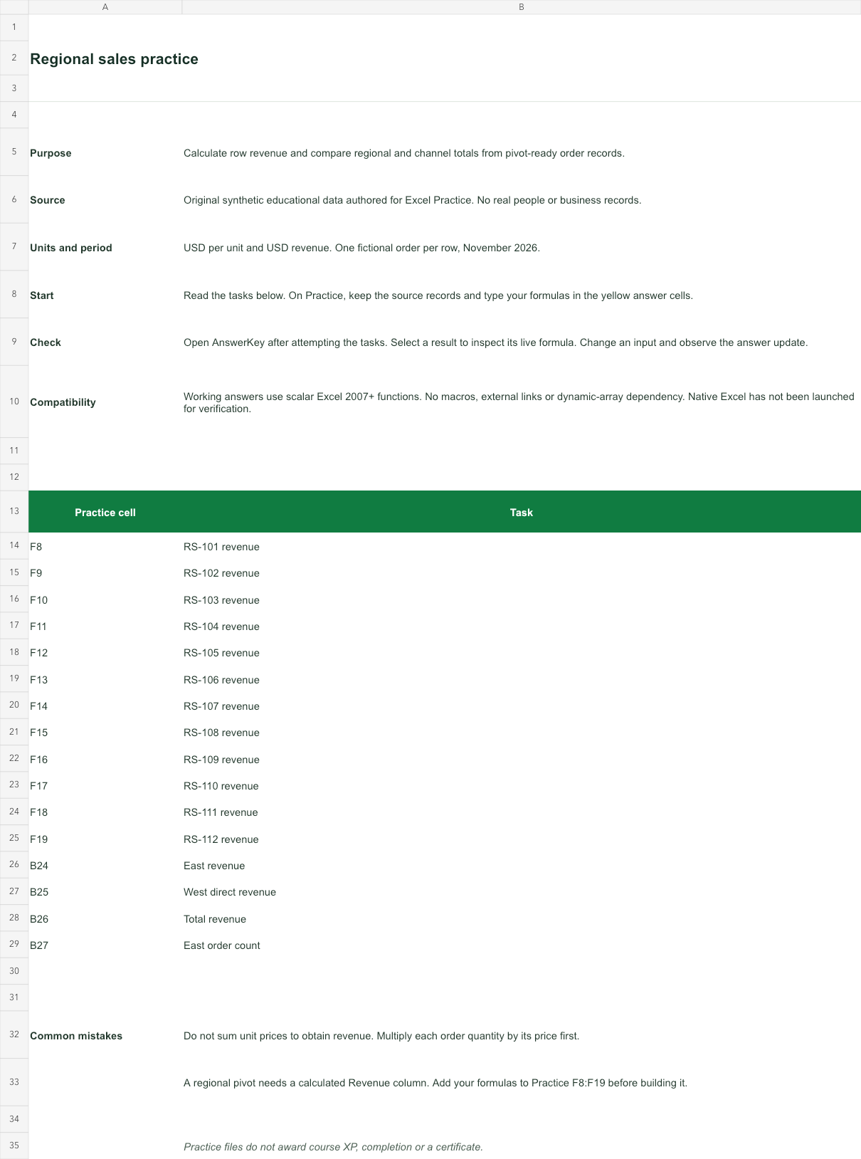
USD per unit and USD revenue. One fictional order per row, November 2026.
Bank version 2026-11-02. Includes Instructions, Practice, AnswerKey; 16 live answer formulas. All source records are invented for education.
The download is an additional practice task. Its Instructions sheet identifies the source coordinates; this page’s illustrative example may use different records.
- Working answers use scalar Excel 2007+ functions. No macros, external links or dynamic-array dependency. Native Excel has not been launched for verification.